A Brief Theory of the Koopman Operator

To understand the Koopman operator, let’s start with the basics. Imagine we have a system of nonlinear differential equations:

\[ \dot{x} = f(x), \]

where:

• \( x \) represents the state of the system (e.g., positions, velocities, or other quantities),
• \( \dot{x} \) is the rate of change of \( x \),
• \( f(x) \) is a potentially nonlinear function that describes how the state evolves over time.

This equation models many systems in nature and engineering, from planetary motion to controlling robots. However, nonlinear systems often exhibit complex, unpredictable behaviors, making them challenging to analyze.

The Koopman Operator: Transforming Nonlinear into Linear

The Koopman operator, denoted as \( \mathcal{K} \), provides a powerful way to study nonlinear systems by shifting our focus from the state \( x \) to observable functions. These observables, \( g(x) \), are functions that describe features of the system state \( x \)—for example:

• The energy of a pendulum,
• The distance of a robot from an obstacle,
• Or other meaningful properties.

The Koopman operator is defined as:

\[ \mathcal{K} g(x) = g(f(x)), \]

where:

• \( g(x) \) is an observable function,
• \( f(x) \) is the nonlinear evolution of the state, as given by \( \dot{x} = f(x) \).

In simple terms:

• Instead of analyzing how the state \( x \) evolves directly, the Koopman operator tracks how features of \( x \) (the observables \( g(x) \)) change over time.
• Remarkably, the Koopman operator is linear in the space of observables, even though the original system dynamics are nonlinear.

This linearity allows us to apply the powerful tools of linear algebra to study complex, nonlinear systems.

Eigenfunctions of the Koopman Operator

An important concept in Koopman theory is the eigenfunction. An eigenfunction \( \phi(x) \) satisfies the following relationship under the Koopman operator:

\[ \mathcal{K} \phi(x) = \lambda \phi(x), \]

where:

• \( \phi(x) \) is the eigenfunction, representing a special observable whose behavior under the Koopman operator is simple—it just scales by a factor \( \lambda \),
• \( \lambda \) is the eigenvalue, which describes how \( \phi(x) \) evolves over time.

In simpler terms: Eigenfunctions are like “building blocks” of the system’s dynamics. They evolve predictably, making them incredibly useful for analyzing and understanding the system.

Why This Matters

The Koopman operator transforms the complex, nonlinear dynamics of the system \( \dot{x} = f(x) \) into a simpler, linear framework by focusing on observables and their evolution. By identifying eigenfunctions and eigenvalues, we can:

1. Decompose the dynamics into simpler, predictable components,
2. Simplify the analysis and prediction of the system’s long-term behavior,
3. Design better control strategies for engineering systems, like robots.

What’s Next?

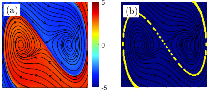
Remember the duffing system from the previous blog post?

Indeed we can characterize the differet regions of the duffing oscillator.

This post explores how density functions define safe navigation by associating high densities with the target and safe regions, low densities with obstacles, and using the positive gradient of the density as a safe path to the goal.

Imagine you’re at a bustling train station during rush hour. People are moving in all directions, suitcases roll past, and announcements echo through the air. Navigating this chaos, you instinctively steer clear of crowded zones, avoiding the hurried travelers and luggage obstacles. Your focus sharpens as you spot a path that feels less congested—a safer route to your platform. Robots face similar challenges in their environments, from crowded warehouses to busy streets. Like us, they must discern safe paths, avoid obstacles, and move toward their goal. This is where density functions come in, giving robots a mathematical lens to identify safe regions and navigate using the positive gradient of density, much like we find our way through a crowd.

What Are Density Functions in Robotics?

Density functions in this context describe the distribution of system trajectories in the robot’s environment:

• High density: Found near the target and safe regions.
• Low density: Found near obstacles and unsafe areas.

Mathematically, the density function \( \rho(x) \) assigns a value to each position \( x \), representing the “attractiveness” of that location. The robot uses this information to navigate by following the positive gradient of the density: \[ \mathbf{u}(x) = \nabla \rho(x), \] where \( \mathbf{u}(x) \) is the robot’s control input (direction of movement), and \( \nabla \rho(x) \) is the gradient of the density function.

How Density Functions Enable Safe Navigation

1. Defining Safe and Unsafe Regions

Density functions provide a spatial map of the environment:

• High-density regions: Indicate areas close to the target or clear of obstacles.
• Low-density regions: Represent unsafe zones near obstacles or hazards.

The robot can interpret this map to distinguish between safe paths and areas to avoid.

2. Following the Gradient

The robot navigates its environment by moving in the direction of the positive gradient of the density function \( \rho(x) \). This means that at every step, the robot seeks to increase the value of \( \rho(x) \), which represents the “density” of safe or goal-oriented regions in the space.

Imagine the density function as a kind of topographic map, where higher values of \( \rho(x) \) correspond to peaks (safe or desirable areas, such as the target location), and lower values represent valleys (unsafe areas, such as obstacles). The robot’s objective is to climb this “density hill,” always heading toward areas with higher density values.

To achieve this, the robot uses the positive gradient of the density function:

• The gradient \( \nabla \rho(x) \) points in the direction of the steepest increase in density at any given point \( x \).
• By following this gradient, the robot ensures it is moving toward regions of increasing density, ultimately reaching the maximum density (the target location).

This strategy not only guides the robot safely toward the goal but also ensures it avoids low-density regions, which are associated with obstacles or unsafe areas. The dynamic nature of the density function allows the robot to adjust its trajectory in real time, ensuring it can adapt to changing environments or unexpected obstacles.

• Naturally steer it toward the target,
• Avoid low-density unsafe regions, ensuring safety.

This is akin to a ball rolling uphill on a potential field, always seeking higher values.

3. Dynamically Adjusting Trajectories

As the robot perceives its environment in real time, it updates \( \rho(x) \) to reflect changes (e.g., a new obstacle appearing). This ensures it always follows the safest, most efficient trajectory to its goal.

A Practical Example

Imagine a robot navigating through a forest to deliver a package. Here’s how density functions help:

1. High density: The area near the delivery point and clear flight paths.
2. Low density: Areas cluttered with trees or other obstacles.
3. Safe navigation: The robot follows the positive gradient of \( \rho(x) \), steering clear of obstacles while moving toward its target.

The high-density regions represent the target, and low-density regions are “no-go” areas where the robot should not go. The gradient of this density function points away from the low-density regions, enabling the robot to course-correct and avoid these regions while navigating toward the target. Next lets see how this can be used to navigate a robot safely through the woods!

Why This Approach Matters

By defining safe and unsafe regions and guiding robots using the gradient of a density function, this approach ensures:

• Safety: Robots naturally avoid obstacles by moving toward higher-density (safe) regions.
• Efficiency: Trajectories are optimized by leveraging a mathematically grounded framework.
• Real-time adaptability: The density function can dynamically adjust based on environmental changes.

This method bridges theoretical insights and practical applications, making it a cornerstone for modern robotic navigation systems.

What’s Next?

In the next post, we’ll explore how to compute the density function in real time using sensor data and integrate it with advanced motion planning algorithms.

But what is the Koopman operator, and why is it so powerful? Let’s explore this concept using a simple analogy—waves on the beach—before diving into how it helps robots navigate a crowded room.

Making Sense of Chaos: Waves at the Beach

Imagine standing on the shore, watching waves crash onto the beach. The motion of the water appears chaotic—every droplet seems to move unpredictably, making it difficult to understand the larger pattern at play. But what if there was a way to shift your perspective, to see the waves not as random splashes but as part of a bigger picture?

It focuses not on the individual droplets but on observable features of the system—like the height, speed, or direction of the waves. These features evolve in time in a way that reveals an underlying order. With this insight, you can predict how the waves will change, even if the motion of each droplet remains complex.

It transforms the way we study dynamic systems, allowing us to understand and predict behaviors that once seemed impossible to decode.

Play with the Waves: See Where the Flow Takes You

Below is a dynamic visualization of how a system (Duffing oscialltor) evolves over time. Imagine you’re watching a drop of water flowing through a twisting, turning river. Click anywhere on the visualization to drop your “water droplet” into the flow and see where it goes. The paths it takes represent how the system behaves from that starting point.

The Duffing oscillator is a classic example of a nonlinear dynamical system that exhibits rich and complex behavior. At its core, the system’s dynamics are shaped by a double-well potential, meaning that there are two stable “wells” where the system can settle, separated by an unstable equilibrium point at the peak of a “hill” between them.

When you click on the visualization to drop your “water droplet,” you’re essentially setting an initial condition for the system. Depending on where you click, the system will flow toward one of the two stable wells or oscillate between them.

Can we use tools like the Koopman operator to understand the different regions of this flow? Check out the next blog post to learn more!

From Waves to Robots: A Real-World Connection

Now, let’s step into a robotics lab. Imagine programming a robot to navigate through a crowded room. People are walking in unpredictable directions, chairs are scattered in different locations, and doors swing open and shut. To the robot, this environment looks as chaotic as the waves at the beach.

But what if the robot could shift its perspective, just like we did with the waves?

How the Koopman Operator Helps Robots

Instead of micromanaging every detail, the robot can focus on observable functions—like:

• The density of obstacles in its path.
• The flow of people toward an exit.

By lifting these features to a higher-dimensional space, the Koopman operator simplifies the robot’s view of the environment. In this lifted space, the dynamics of the room often become linear and easier to predict, enabling the robot to make smarter, faster decisions.

Why It Matters

The Koopman operator bridges the gap between chaos and clarity. It allows us to move from the unpredictable motion of individual elements to the predictable evolution of patterns. Whether it’s understanding waves or programming robots, this mathematical tool reveals the hidden order in the systems around us.

Next Steps

In the next section of this blog, we’ll dive deeper into the mechanics of the Koopman operator, explore how it works in practice, and look at real-world applications that bring this concept to life. Also check out how we can use density functions to help robots navigate safely.

If you have any questions or would like to learn more, feel free to leave a comment below!