
Navigating Safely: Following the Path of Density
Published:
Robots today are more than machines; they’re companions, assistants, and explorers. For these robots to safely navigate dynamic and cluttered environments—like a robot vacuum avoiding toys or a delivery drone dodging pedestrians—they need a clear understanding of their surroundings. One powerful tool they use is density functions, a mathematical framework to represent safe and unsafe areas while guiding them safely toward their goals.
This post explores how density functions define safe navigation by associating high densities with the target and safe regions, low densities with obstacles, and using the positive gradient of the density as a safe path to the goal.
Imagine you’re at a bustling train station during rush hour. People are moving in all directions, suitcases roll past, and announcements echo through the air. Navigating this chaos, you instinctively steer clear of crowded zones, avoiding the hurried travelers and luggage obstacles. Your focus sharpens as you spot a path that feels less congested—a safer route to your platform. Robots face similar challenges in their environments, from crowded warehouses to busy streets. Like us, they must discern safe paths, avoid obstacles, and move toward their goal. This is where density functions come in, giving robots a mathematical lens to identify safe regions and navigate using the positive gradient of density, much like we find our way through a crowd.
What Are Density Functions in Robotics?
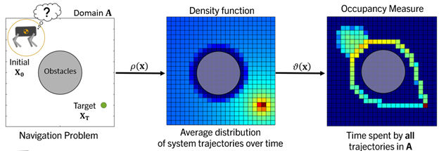
Density functions in this context describe the distribution of system trajectories in the robot’s environment:
- High density: Found near the target and safe regions.
- Low density: Found near obstacles and unsafe areas.
Mathematically, the density function \( \rho(x) \) assigns a value to each position \( x \), representing the “attractiveness” of that location. The robot uses this information to navigate by following the positive gradient of the density: \[ \mathbf{u}(x) = \nabla \rho(x), \] where \( \mathbf{u}(x) \) is the robot’s control input (direction of movement), and \( \nabla \rho(x) \) is the gradient of the density function.
How Density Functions Enable Safe Navigation
1. Defining Safe and Unsafe Regions
Density functions provide a spatial map of the environment:
- High-density regions: Indicate areas close to the target or clear of obstacles.
- Low-density regions: Represent unsafe zones near obstacles or hazards.
The robot can interpret this map to distinguish between safe paths and areas to avoid.
2. Following the Gradient
The robot navigates its environment by moving in the direction of the positive gradient of the density function \( \rho(x) \). This means that at every step, the robot seeks to increase the value of \( \rho(x) \), which represents the “density” of safe or goal-oriented regions in the space.
Imagine the density function as a kind of topographic map, where higher values of \( \rho(x) \) correspond to peaks (safe or desirable areas, such as the target location), and lower values represent valleys (unsafe areas, such as obstacles). The robot’s objective is to climb this “density hill,” always heading toward areas with higher density values.
To achieve this, the robot uses the positive gradient of the density function:
- The gradient \( \nabla \rho(x) \) points in the direction of the steepest increase in density at any given point \( x \).
- By following this gradient, the robot ensures it is moving toward regions of increasing density, ultimately reaching the maximum density (the target location).
This strategy not only guides the robot safely toward the goal but also ensures it avoids low-density regions, which are associated with obstacles or unsafe areas. The dynamic nature of the density function allows the robot to adjust its trajectory in real time, ensuring it can adapt to changing environments or unexpected obstacles.
- Naturally steer it toward the target,
- Avoid low-density unsafe regions, ensuring safety.
This is akin to a ball rolling uphill on a potential field, always seeking higher values.
3. Dynamically Adjusting Trajectories
As the robot perceives its environment in real time, it updates \( \rho(x) \) to reflect changes (e.g., a new obstacle appearing). This ensures it always follows the safest, most efficient trajectory to its goal.
A Practical Example
Imagine a robot navigating through a forest to deliver a package. Here’s how density functions help:
- High density: The area near the delivery point and clear flight paths.
- Low density: Areas cluttered with trees or other obstacles.
- Safe navigation: The robot follows the positive gradient of \( \rho(x) \), steering clear of obstacles while moving toward its target.
The high-density regions represent the target, and low-density regions are “no-go” areas where the robot should not go. The gradient of this density function points away from the low-density regions, enabling the robot to course-correct and avoid these regions while navigating toward the target. Next lets see how this can be used to navigate a robot safely through the woods!
Why This Approach Matters
By defining safe and unsafe regions and guiding robots using the gradient of a density function, this approach ensures:
- Safety: Robots naturally avoid obstacles by moving toward higher-density (safe) regions.
- Efficiency: Trajectories are optimized by leveraging a mathematically grounded framework.
- Real-time adaptability: The density function can dynamically adjust based on environmental changes.
This method bridges theoretical insights and practical applications, making it a cornerstone for modern robotic navigation systems.
What’s Next?
In the next post, we’ll explore how to compute the density function in real time using sensor data and integrate it with advanced motion planning algorithms.